Synthetic Testing in AWS: Challenges and Solutions
A bare-metal server versus a cloud server: not a dilemma anymore. Specialists know that both have their pros and cons, and they make the choice depending on each client’s needs. Clients, however, are not always aware of the risks of cloud migration.
Also, they often believe that by paying the provider of cloud services the same amount of money as other clients do, they will get the same hardware behind the cloud. One of the greatest risks, however, is that you don’t actually know the system’s limitations. By testing your system in the cloud, you can avoid most migration risks and save money in the long run. Wild Apricot is a case in point.
Table of Contents
Load Profile for Synthetic Testing in AWS
Our client is powerful cloud software that helps automate and simplify membership tasks. It is based in Toronto, Canada, and has held the top spot in the Membership Management Software ratings for many years in a row.
Back in 2016, they decided to move their systems entirely to the cloud. With 6 million users and 15 k communities (i.e., websites, each with a unique design and its own events and fundraisers, blogs, and forums), the migration risks were high. PFLB helped them get it done.
The Task: Synthetic Testing in AWS
Wild Apricot wanted to seamlessly move everything to cloud hosting and chose AWS as the platform. The objective was to cut maintenance costs, increase availability up to 100%, and ensure the scalability of services in cloud computing.
To confirm that cloud migration made sense, we had to:
- run performance testing in a cloud environment
- run synthetic testing in AWS
- configure the monitoring system
It seemed ordinary, but it was not.
Load Profile for Synthetic Testing in AWS
As soon as we started, we faced a couple of challenges. First, we got 50 GB of IIS server logs PER MONTH to process to build the load profile. Obviously, we should have told the client which logs we needed, but we hadn’t. We had neither that much server power nor the time or money to buy additional servers. So, we improvised. We used PowerShell to get rid of useless data from the logs and reduced the overall volume by 50%. We processed the remaining half with Python, grouped the data, and further filtered out any unnecessary data.
The next step was to group the actions by the appropriate time frame. We needed it with 1-minute — in some cases even 1-hour — granularity, depending on the particular task. However, the source data were logged every second. Once done, we processed the data again with our own library and Pandas to get the final result. The load profile was beautiful, and it only took us 2 days to process the logs.
AWS Monitoring Systems: Challenges and Results
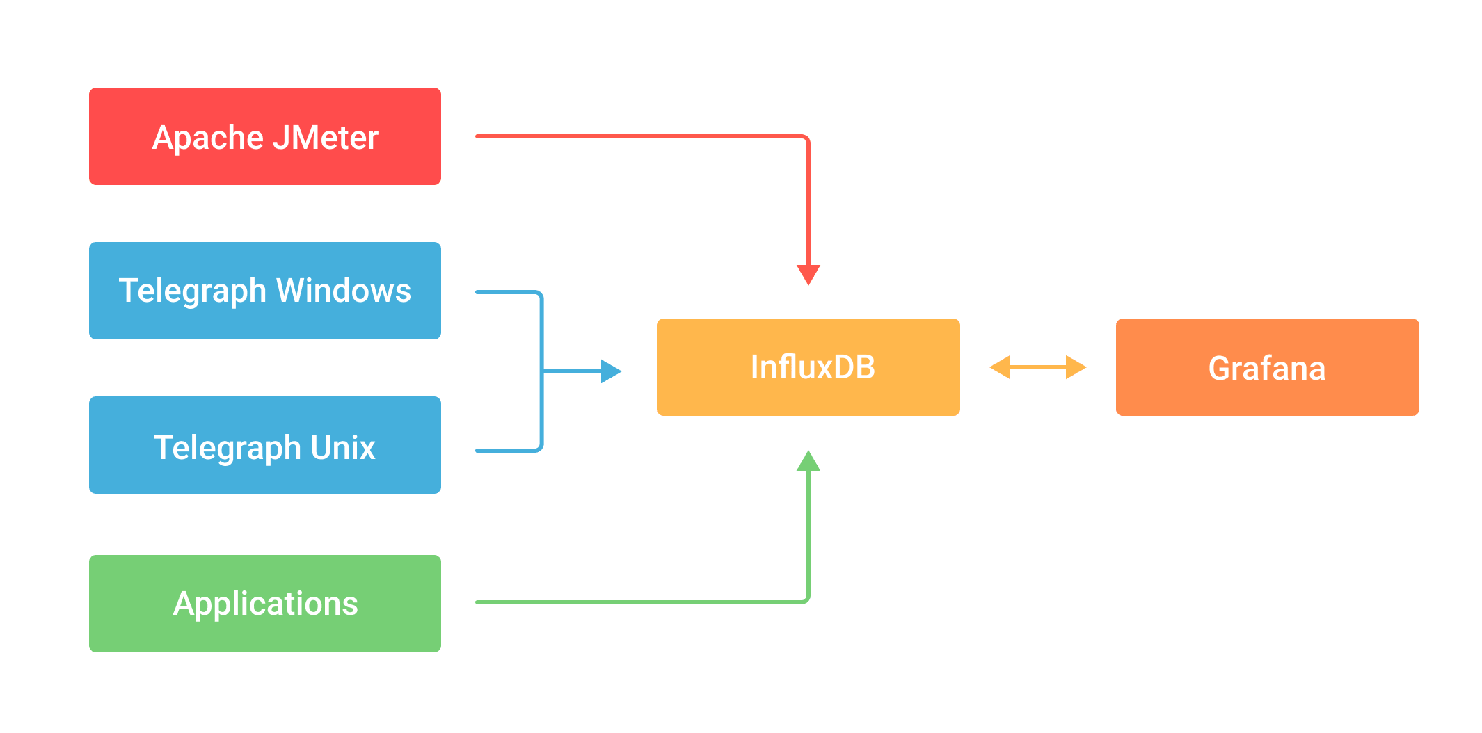
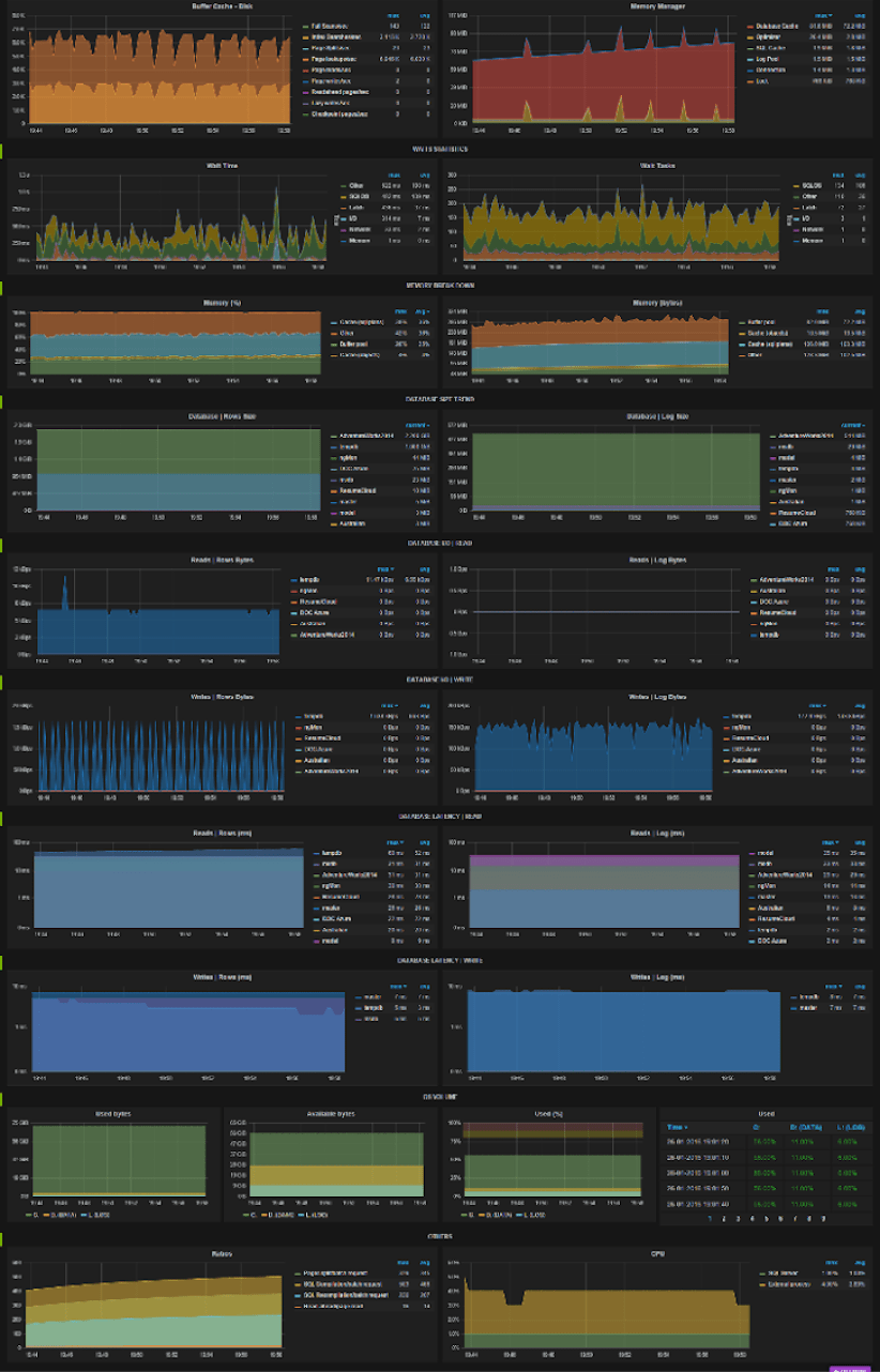
We used InfluxDB to combine the monitoring data, Grafana to visualize it, and Telegraph to monitor hardware resource utilization and app performance. We did our best to keep everything in-cloud and online, and the combination of these monitoring solutions seemed fine for the cloud, too.
One of the challenges of monitoring was that we were changing the data sources all the time—both instances and load generators. We were constantly stopping the running ones and introducing new ones to simulate new circumstances and increase the load. Obviously, we had to embed Telegraph into the images of all the stations.
As a new instance was spun up, it started the listener and posted the data to the database. In the end, we had 7 Telegraph configurations in 29 constantly working instances—plus three load stations and one more for monitoring. This added up to 11 dashboards in Grafana, each with its own graphs.
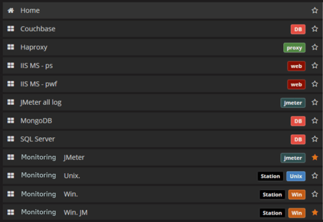
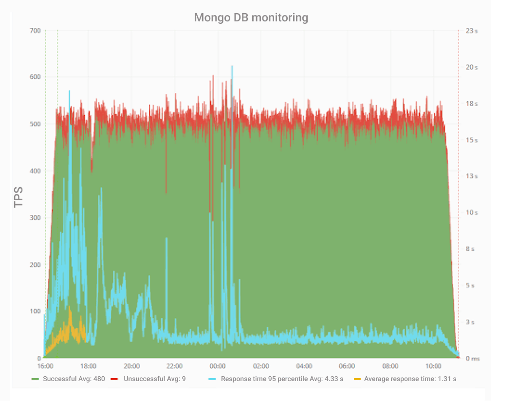
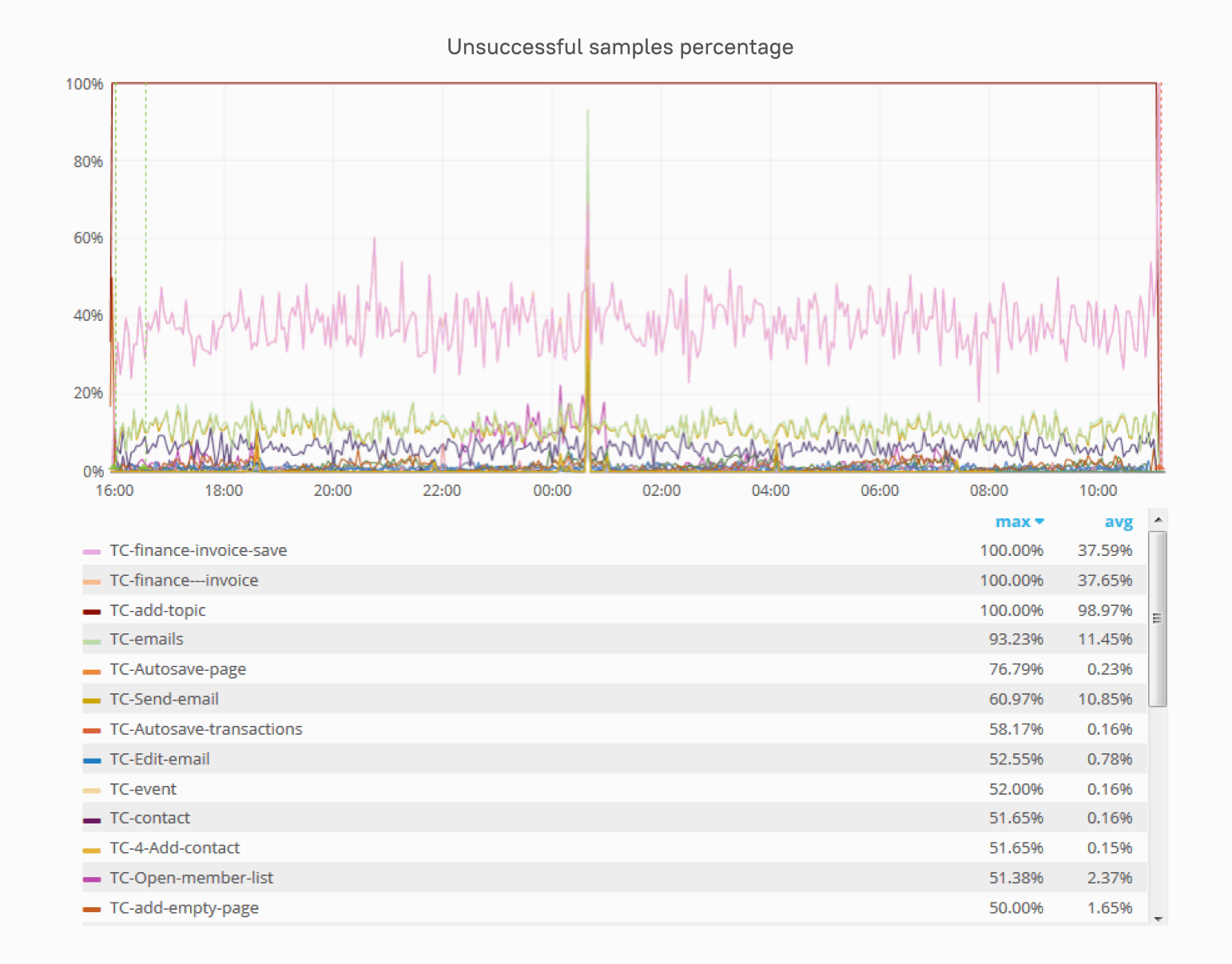
Plus, we were monitoring JMeter separately. We gathered TPS, errors, response times, and other custom metrics. Look at the graphs for MongoDB and MSSQL. Aren’t they beautiful? And informative, too: you can take a closer look at every single phase.
But we had a problem—in fact, more than one. Twenty-nine servers sending out metrics every minute, multiplied by, say, 12 hours of load testing is a massive—in this case, overwhelming—amount of data. Unfortunately, Grafana limits the amount of data that can be presented in one graph. Due to these limitations, you simply can’t see the results. It’s either 1 server x 12 hours or 29 servers x 1 hour.
Also, Grafana shows the graphs in your browser, and it gets too slow with growing amounts of data. We had to optimize it to make it load all the graphs simultaneously. First, we optimized the queries sent from Grafana to InfluxDB. Then, we hid the graphs that weren’t used very often to make only what we really needed visible. We also configured alerts and put them on the alert list. We configured Grafana to send screenshots along with an alert when it was triggered to Telegram, but instead you could use e-mail or any messenger of your choice. This way, you won’t need to constantly follow each and every graph, as we did at first.
Synthetic Testing: Our Approach
Eventually, we had to choose synthetic testing software for AWS. The key factor was that the solutions had to be cross-platform, as some servers ran on Linux, while others used Windows. Of course, you’d also like the software of your choice to be free and as fast as possible yet yield explicit results. The final list was as follows:
- Linpack for the CPU
- pmbw for memory
- iPerf3 for the network
- fio for the hard disk (although it soon turned out that fio needs a very specific sequence in AWS).
The next step was to figure out the metrics, since without them the test lasted 8 hours. Unacceptable, right? But the client wanted to run synthetic tests before starting the process of adding each machine to the pool of working ones to ensure that it was as functional as any. We chose matrix size for the CPU and block size for the disk, as well as interaction types, such as reading/writing and randomized access. With the metrics, the test took only half an hour.
Want to Learn More about Our Performance Testing Services?
Find out what’s included and how to start working with us
Synthetic Testing: Troubleshooting
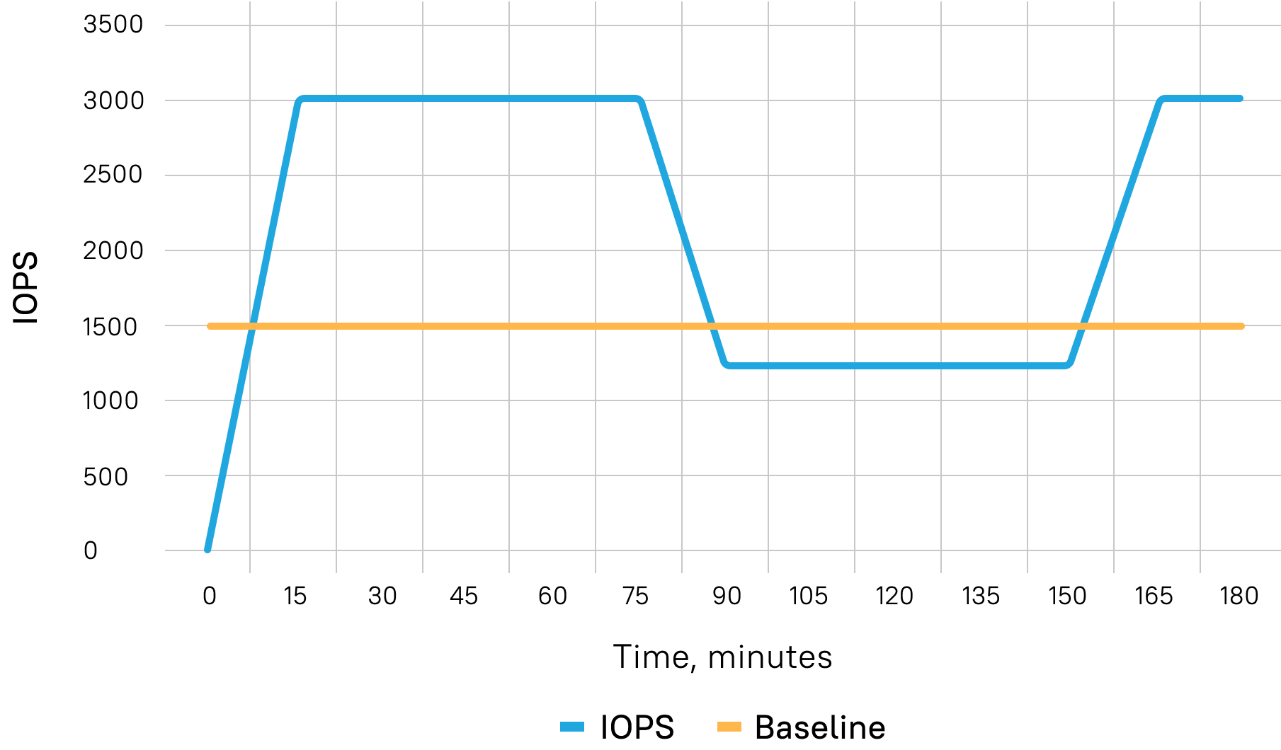
But there was another obstacle. Suddenly, it just looked too good—too quick, with results unrealistic for synthetic testing in AWS. The thing is, AWS has this undocumented, top-secret feature that would ruin any test. It’s called Burst. With Burst, your results look better than perfect. Each of your hard disks gets a credit of 5 million IOPS for about 30 minutes. This credit allows you to use many more IOPS than you paid for (as many as 5 million!), and all applications start smoothly, quickly, and simultaneously. However, after the credit has been used, the IOPS are set back to the previous level. Then, when you go lower than the baseline, which is around 1500 IOPS, the credit starts growing again. The exact numbers, of course, depend on the hard disk type, volume, etc. To overcome this performance challenge, which had to do particularly with cloud computing, we had to exhaust Burst every time to prepare the system before running the load tests. This point is crucially important; your tests will otherwise be useless.
The challenges we encountered later on also influenced the load testing process. First, we needed to randomize the sequence in which Apache JMeter picked lines from the file with site addresses—specifically, 5800 of them. Unfortunately, by default, it can only read them sequentially. To randomize the order, we used the HTTP Simple Table Server JMeter plugin. If you are experiencing similar problems with your performance testing in a cloud environment, we highly recommend that you do the same. If we had used it from the start, it would have saved us a lot of time.
Still, with 5800 separate sites, we kept running out of available connections. Buying more was not an option, since we were in the cloud. You can’t just add an extra memory module to your machine. You’d have to change the instance and pay for it not once but every time. There was no other option but to tune the load station. We changed the following parameters on one machine to increase the number of connections:
- MaxUserPort – number of free ports
- TcpTimedWaitDelay – socket wait duration
- TcpFinWait2Delay – amount of time needed to keep a half-closed connection
This helped for a while, but then the test crashed again. A final move was to switch off keep-alive in scripts because most of the time, the tests did not return to the same site. Once again, problem solved.
The last issue was memory leaks. JMeter leaked around 6 GB per hour—and in AWS, you have to fight for every gigabyte. It is advertised all over the internet that scaling in AWS is easy, but this is just not true. We configured monitoring for the Java Virtual Machine by connecting the Java agent to JMeter and then retrieved the memory dump and analyzed it. We found that the HTTP request classes were taking up most of the memory, as they collect all the request information but are not discarded by the garbage collector. That’s why there were memory leaks.
The Java agent data were sent directly to the database and monitored in real time in Grafana. This allowed us to immediately evaluate the changes we had made in the Java Virtual Machine and in the script instead of just waiting for another crash.
Conclusions: Bare Metal or Cloud After All?
The parameters and configurations in a cloud are very different from those in the same hardware accessed outside a cloud. There are many details to consider. The system didn’t work the first or second time we started it, but with the 8th iteration, we succeeded.
We saved the client a lot of time, money, and nerves, took new approaches, and used new JMeter functionalities that eased our work tremendously. During testing, we chose the best AWS hardware configuration for the client’s system. Performance and scalability in cloud computing are different, but this does not mean that they are worse. To avoid the risks, however, you should run the tests.